Views reference

One section per sidebar view. Unless a caption says otherwise, each screenshot is the bundled synthetic example in browser preview; the values are illustrative, not GPU measurements.

One rule applies to every view: no metric or diagram below is evidence that unobserved CUs, spills, bank conflicts or graph replays are zero. "Not collected" is always shown distinctly from an observed numeric zero. See Limits & caveats.

ISA reference

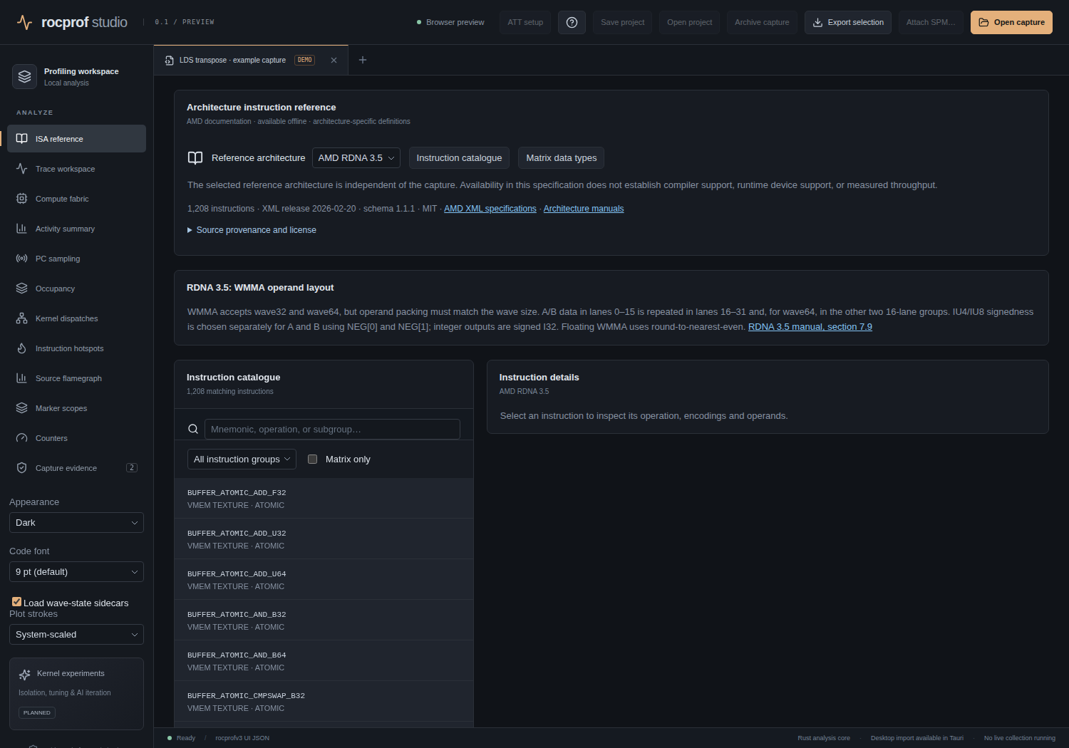
An offline catalogue of AMD instruction definitions for CDNA 1–4 and RDNA 1/2/3/3.5/4 (≈10,628 entries): encodings, operand formats, and WMMA/MFMA/SWMMAC/SMFMAC matrix-type compatibility. It is searchable and is reachable from a selected trace instruction via Instruction reference. The data is regenerated with scripts/build-isa-reference.py.

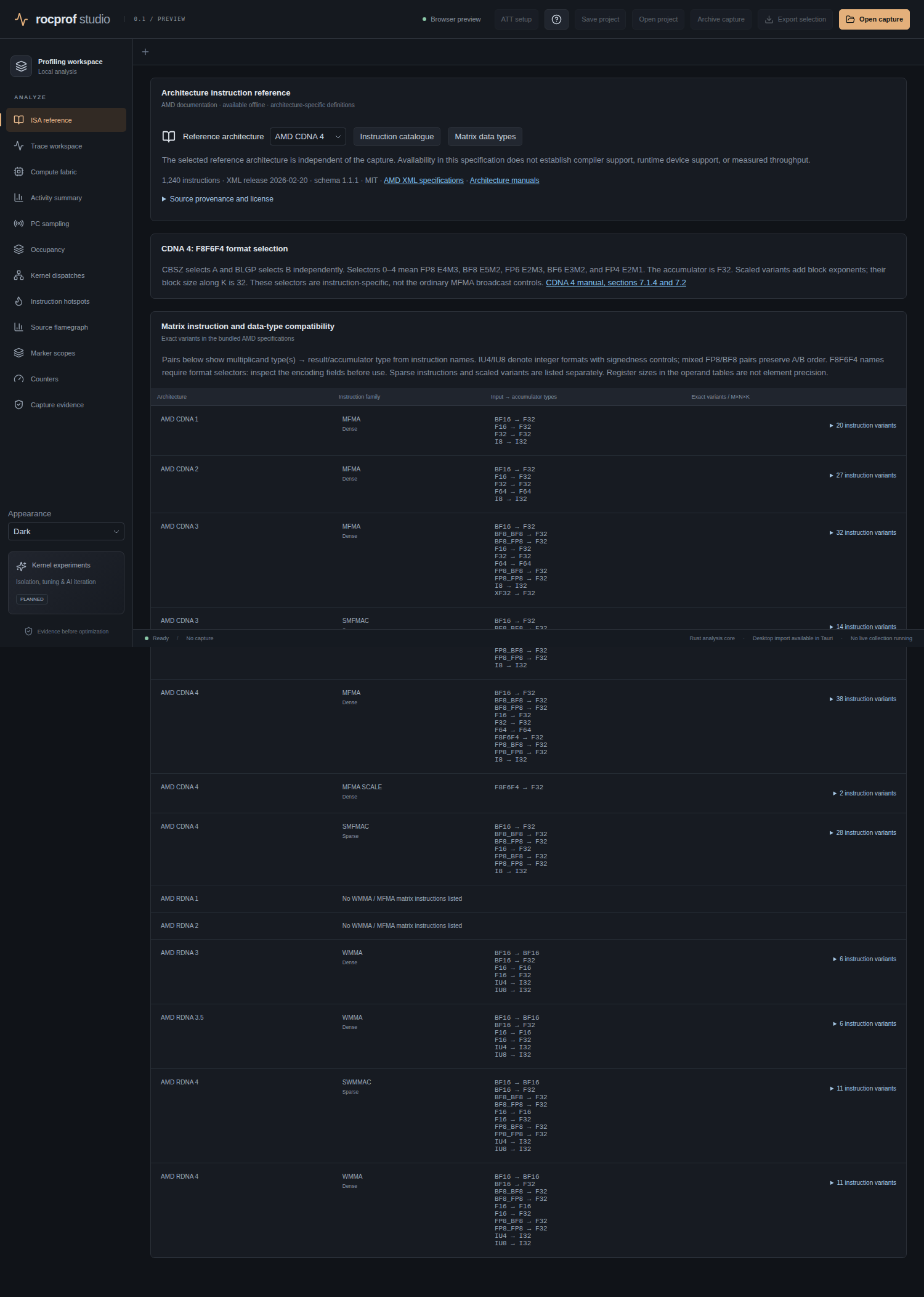The matrix-type compatibility matrix.

Trace workspace

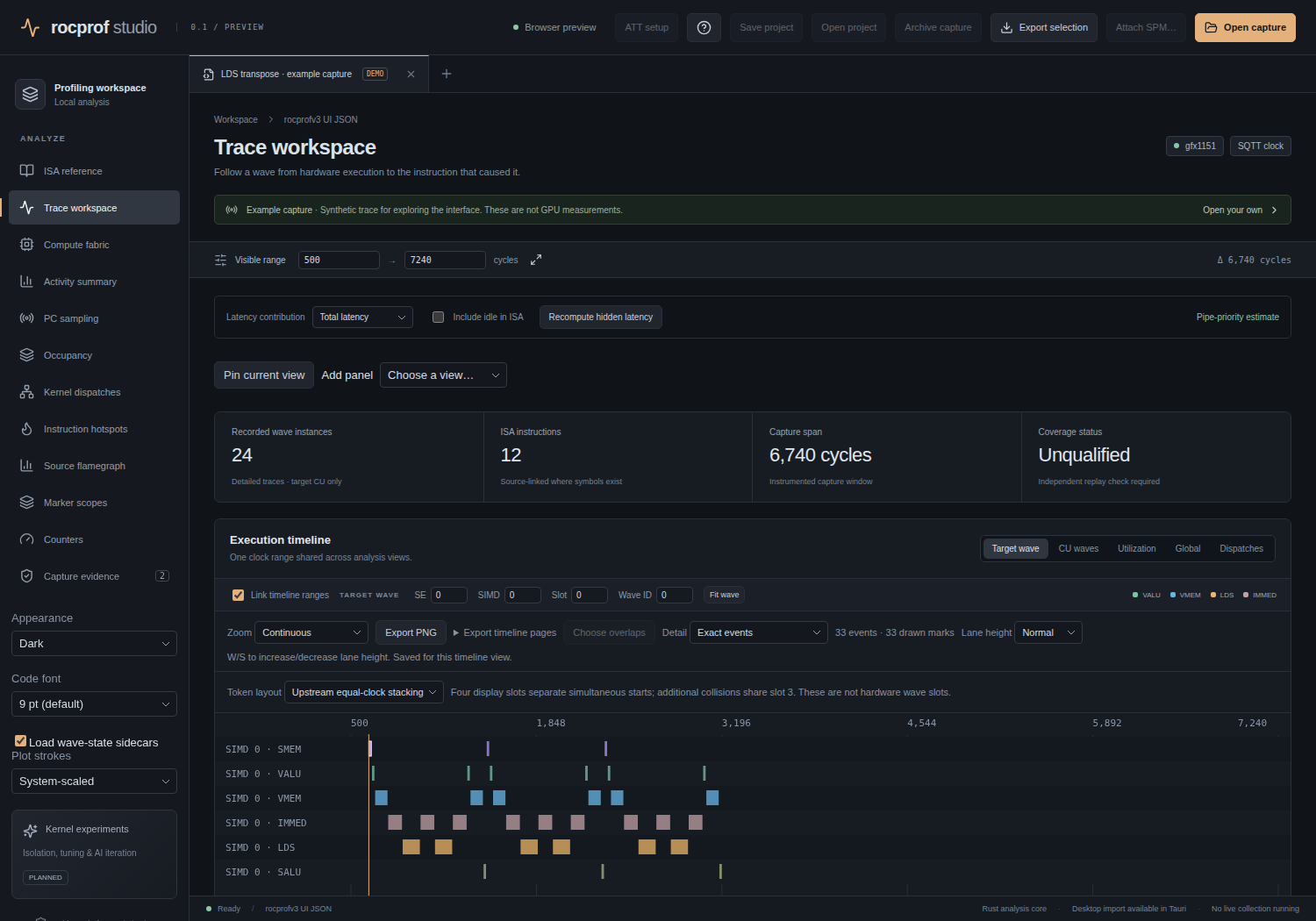
The core view: the execution timeline over five projections (Target wave by instruction class, CU waves by SIMD/slot, SIMD utilization, Global residency, Dispatch timeline), with a linked ISA explorer and Source snapshot underneath.

What the numbers mean:

• Recorded wave instances / ISA instructions / Capture span summarise the capture; Coverage status reads "Unqualified · Independent replay check required" because coverage cannot be proven from the import alone.
• In the ISA table, Hits is the number of recorded executions of that instruction, Cycles the attributed cost under the current latency scope, Stall the stalled portion, and PC samples the sampling hits where available. The Latency scope selector switches between whole-capture sum/mean, target-wave maximum/selected-occurrence, and visible-range sums/means.
• The Source snapshot overlays per-line cost. "Inline locations are inclusive; one instruction can contribute to multiple lines. An em dash means no recorded value; ≥ marks a partial sum." Wait dependencies are reconstructed from named counters when imported links are absent.

Compute fabric

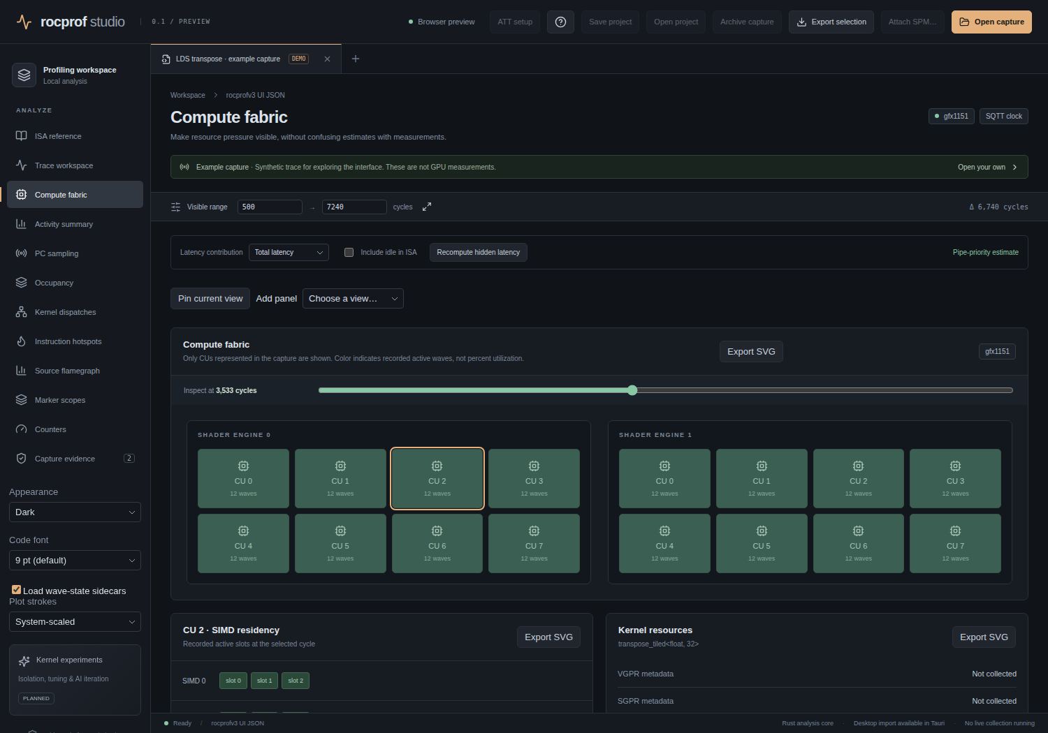
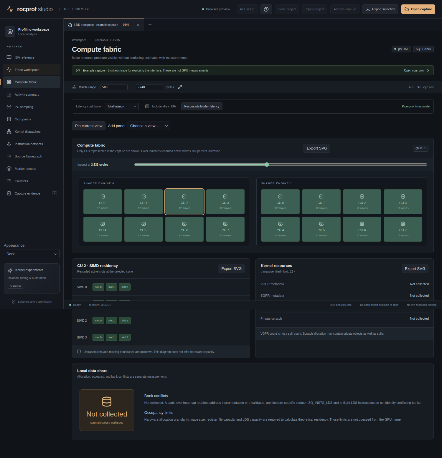
A CU/SIMD residency diagram plus static register/LDS metadata, with explicit unknown states where a value was not recorded. Use it to see which compute units a dispatch actually occupied.

Activity summary

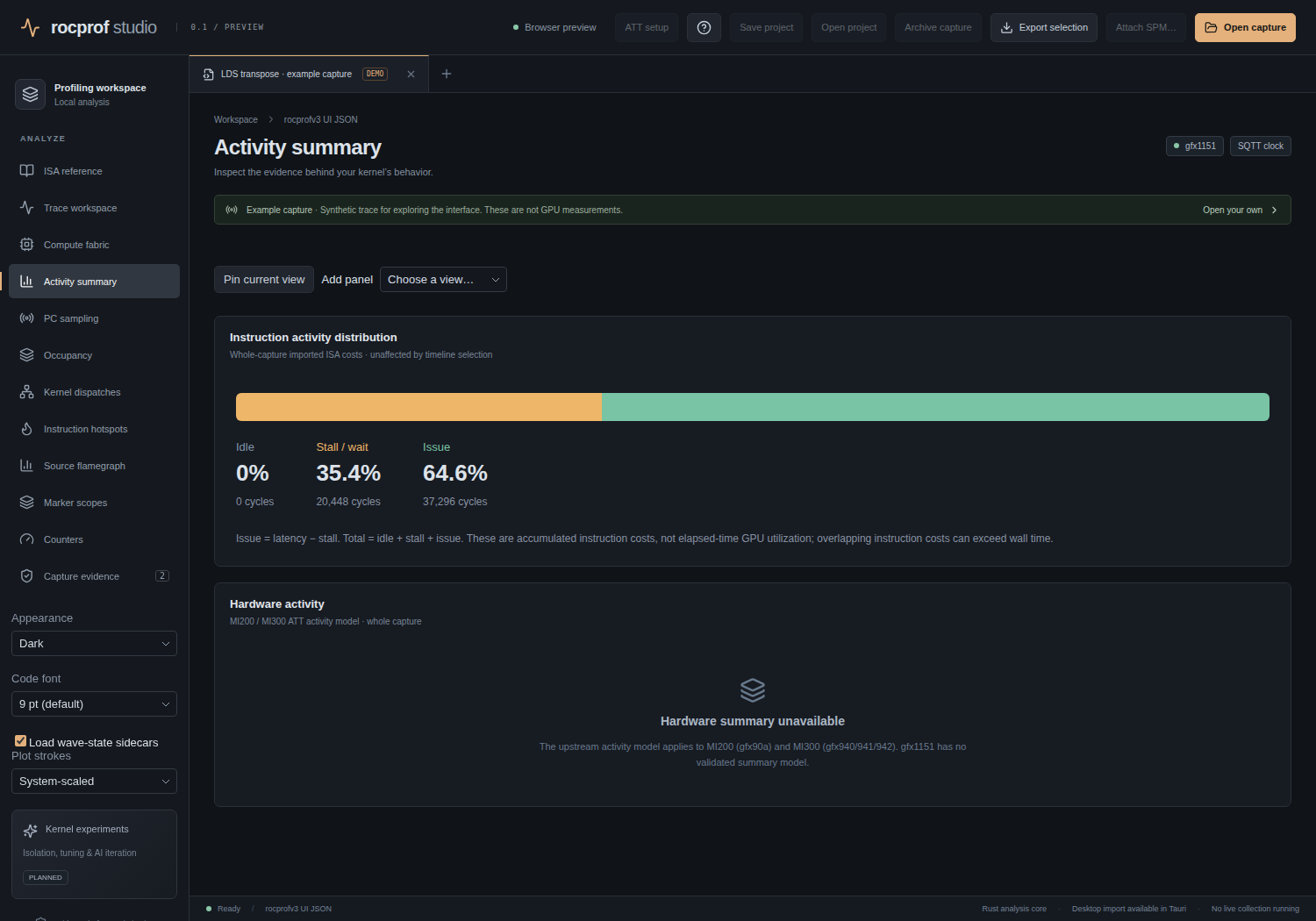
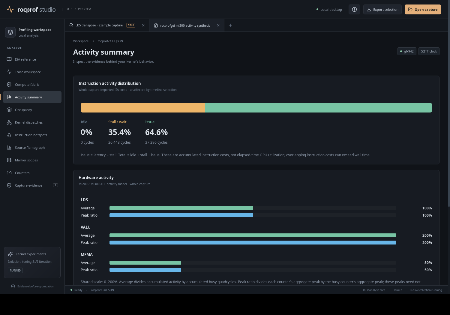
Activity cost plus a hardware-activity model (MI200/MI300 ATT activity bars, peak ratios) and a per-CU table. The hardware-activity model runs in a Web Worker; on an unsupported architecture, a missing ATT counter, or an input above the sample cap it falls back to a synchronous path and reports the limitation rather than guessing. Input is capped at 2,000,000 samples.

PC sampling

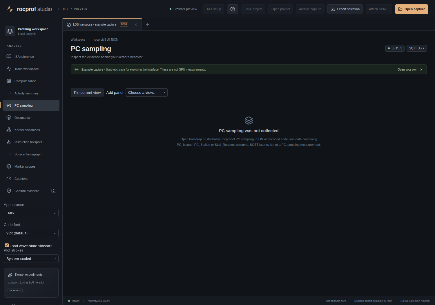
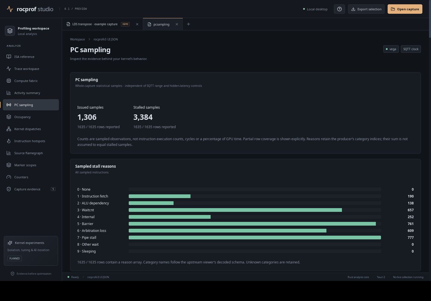
Totals, stall-reason breakdown and a flamegraph for host-trap or stochastic PC-sampling data. Host-trap and stochastic samples are kept as distinct identities; raw observation rows are searchable.

Occupancy

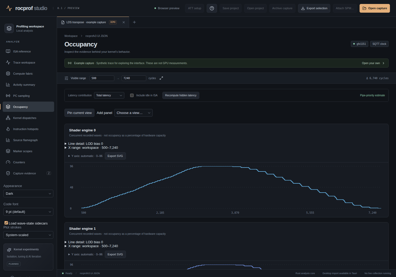
Per-SE and per-kernel occupancy plots: how many waves were resident over time. Export is available as SVG.

Kernel dispatches

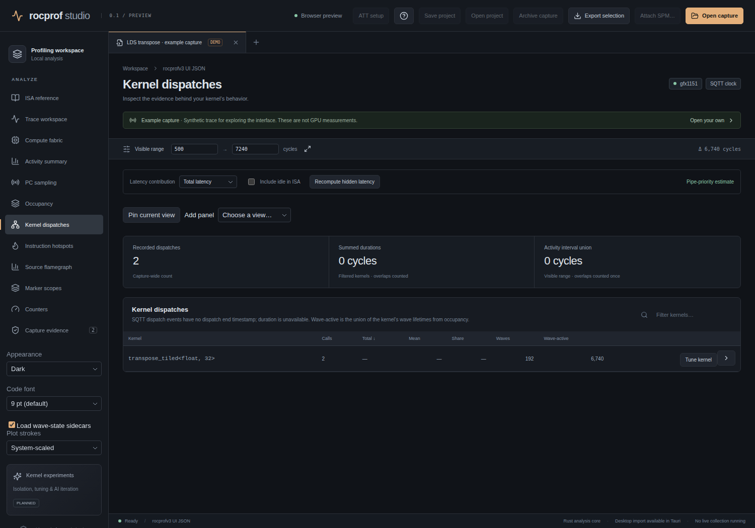
The dispatch list/timeline with host-API call association. This view reports summed durations and interval union separately, because kernel intervals overlap and those two numbers answer different questions (total work vs wall-clock span). See Export & evidence. A selected dispatch is also where "Tune this kernel" (Kernel tuning) is offered.

Instruction hotspots

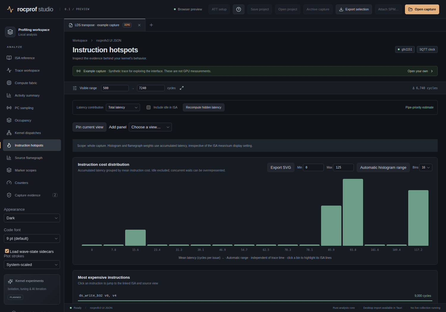
Instruction-cost histograms with an independent mean-latency axis: which instructions dominated, by hits and by cost.

Source flamegraph

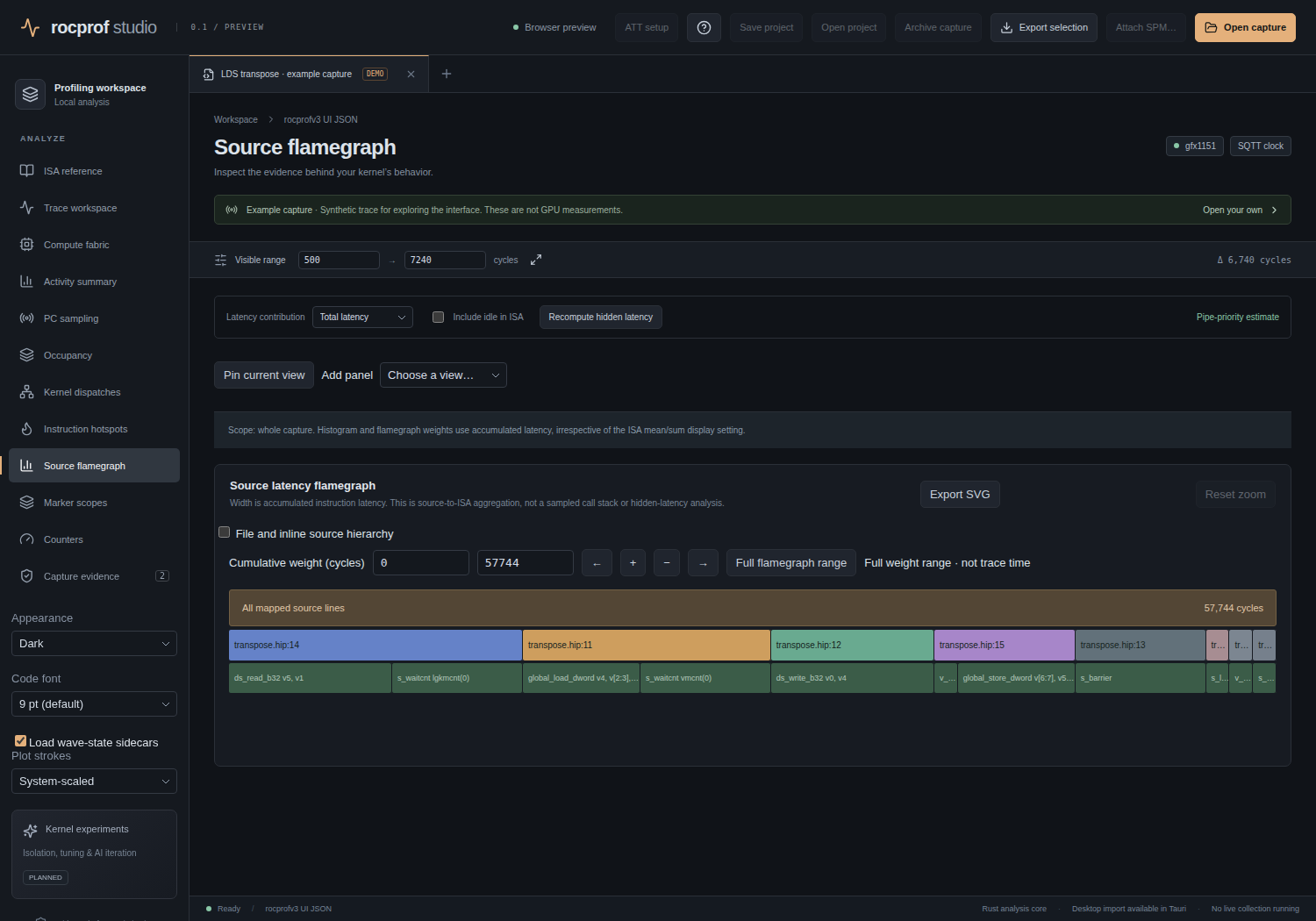
A source-to-ISA latency flamegraph: cost rolled up through the source hierarchy. The viewport is sampled for responsiveness, and above its budget it refuses rather than silently downsampling.

A Group by control groups the flamegraph by source location (the default) or by code object — the compiled kernel unit, which is a pipeline/kernel label for RADV captures and the ELF code-object id for HIP/ATT captures. Code-object grouping is the honest per-kernel dimension this summed aggregate supports: each instruction carries exactly one code object, and an empty one is shown as Unknown code object rather than guessed. It is not a per-dispatch cost split; for true per-dispatch source cost on RADV captures, use the Marker scopes hierarchy. Both groupings remain source-to-ISA aggregation, not a call stack or a time axis. The choice is saved per capture, each grouping keeps its own viewport, and the SVG export caption records which produced it.

Marker scopes

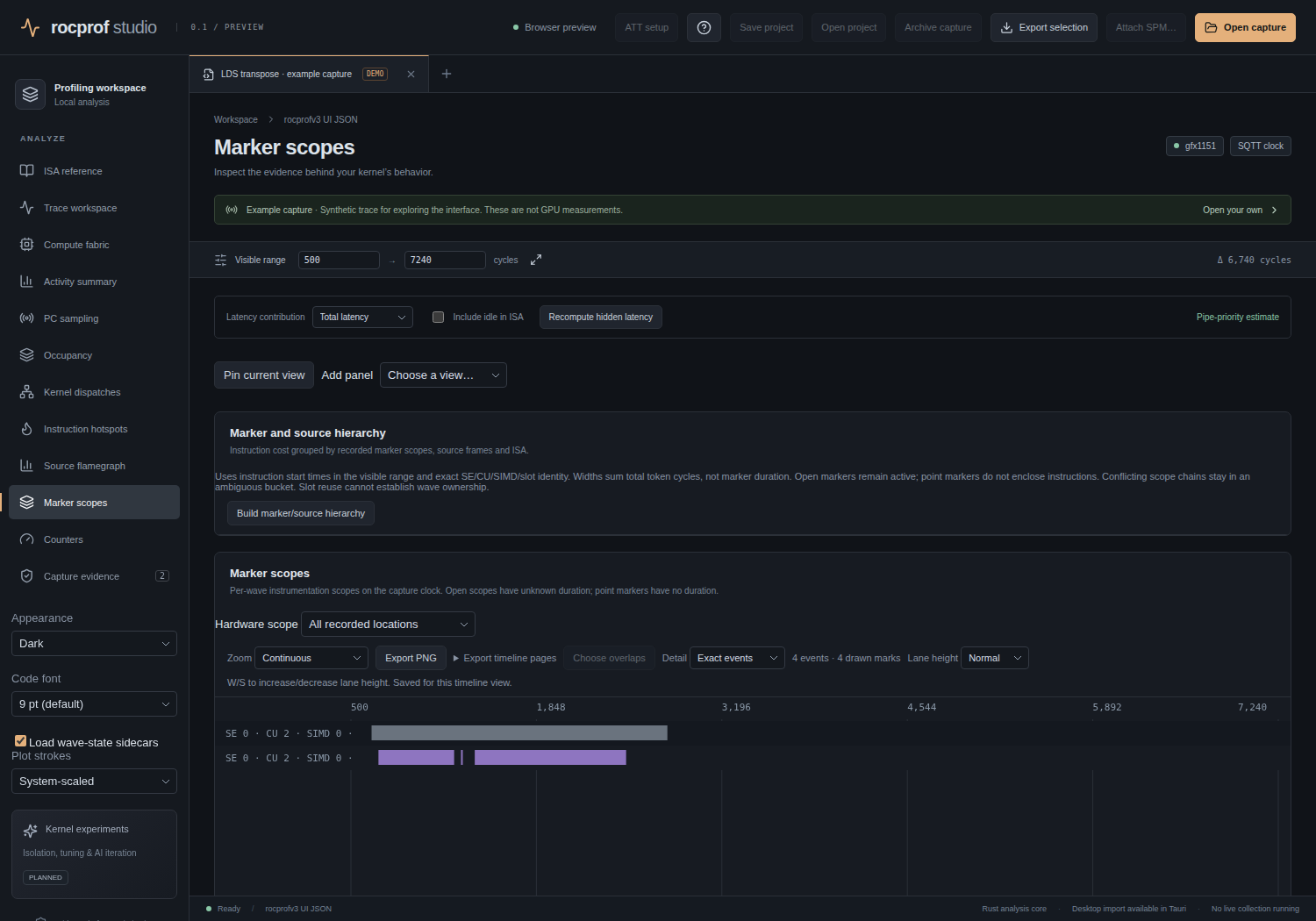
An instrumentation-marker timeline and flamegraph with an integrated marker → source → ISA hierarchy and a separate cumulative-duration viewport.

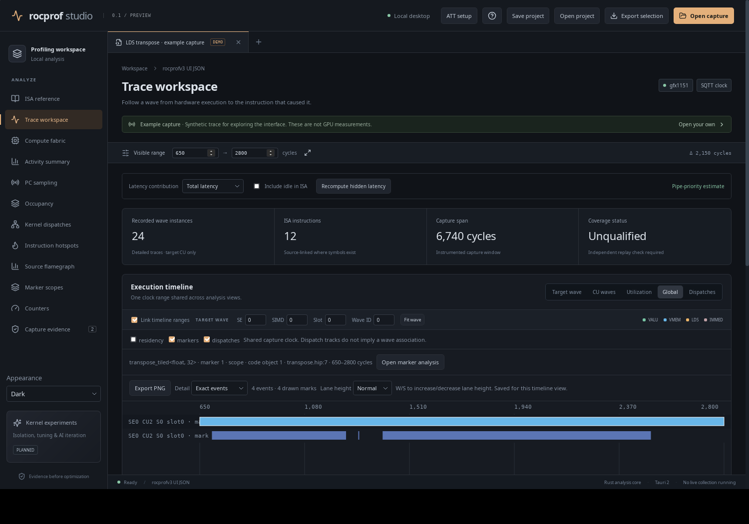Marker overlays on the global timeline (desktop app).

Counters

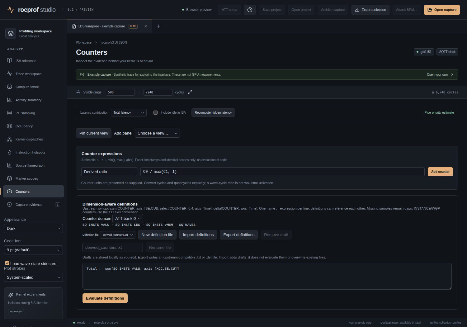
Two kinds of counter work:

• Scalar expressions (Add counter): safe arithmetic over recorded counters (C0, …). Up to 64 definitions per capture; synchronous evaluation over up to 500,000 samples.
• Named-axis tensor definitions: reductions, broadcasting, slices/deltas, comparisons, temporary variables, and a multi-file definition library. These run in a Web Worker with hard caps (1,000,000 input samples, 4,000,000 raw cells, …; see Limits) and a 30-second timeout; exceeding a cap throws.

Raw counter series keep their names and scopes; no architecture-derived normalization is guessed.

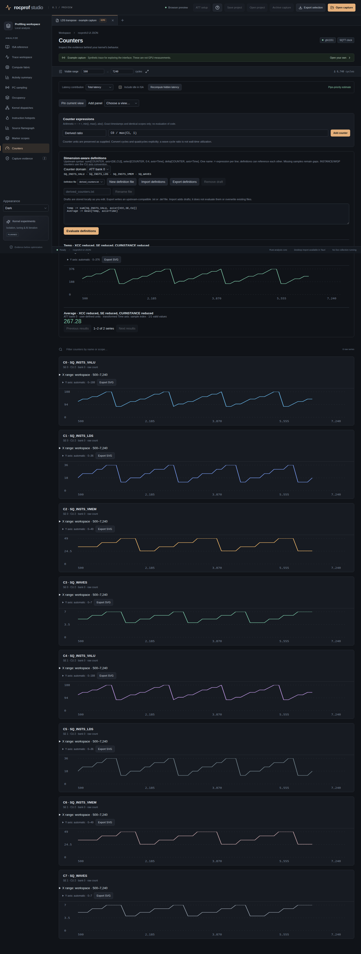Scalar counter expressions in the desktop app.

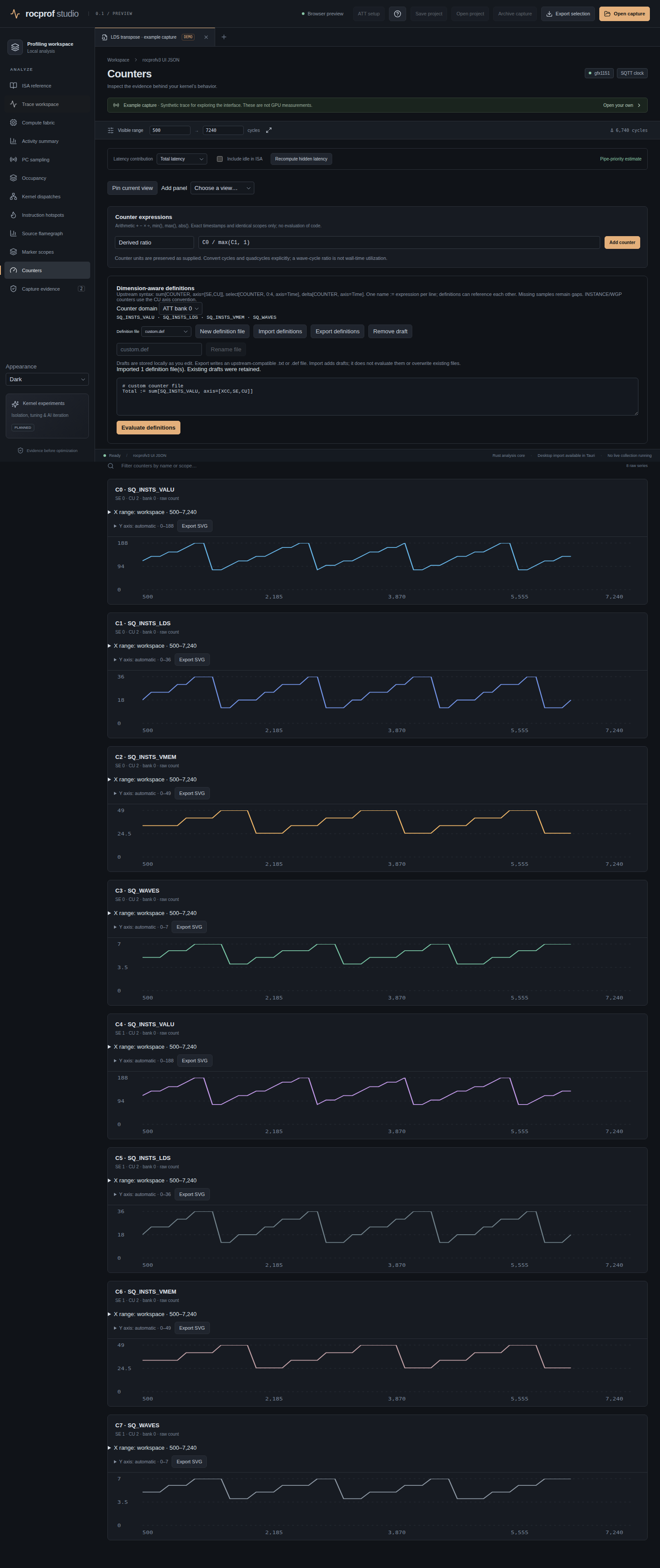The multi-file counter-definition library.

Capture evidence

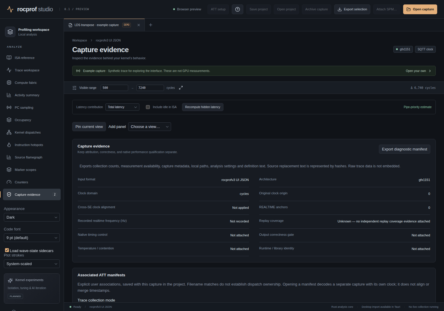
The honesty surface: capture warnings, code-object list with byte-range extraction and relocations, trace↔dispatch associations, coverage diagnostics, and the export actions (diagnostic manifest, selection JSON, SVG/PNG, archive). Covered in detail in Export & evidence.